DataCorrelations-LinearRegression
Housing Prices
Course: MGOC15 - Introductory Business Data Analytics
Topics Tested: Data Correlations, Linear Regressions
Given Data: The data provides the sale prices of different homes in a small town in Iowa, USA.
Final objective is to use linear regression to predict the house prices as accurately as possible, understanding what drives housing prices and how potential home owners value different features of a house.
The data contains the following variables:
Id: Unique ID of property
Neighborhood: Physical locations within city
LotFrontage: Linear feet of street connected to property
Street: Type of road access to property
   Grvl	Gravel
   Pave	Paved
Total_sqr_footage: Total size of the house in square feet
BldgType: Type of dwelling
   1Fam	Single-family Detached
   2FmCon	Two-family Conversion; originally built as one-family dwelling
   Duplx	Duplex
   TwnhsE	Townhouse End Unit
   TwnhsI	Townhouse Inside Unit
OverallQual: Rates the overall material and finish of the house
   10	Very Excellent
   9	Excellent
   8	Very Good
   7	Good
   6	Above Average
   5	Average
   4	Below Average
   3	Fair
   2	Poor
   1	Very Poor
OverallCond: Rates the overall condition of the house
   10	Very Excellent
   9	Excellent
   8	Very Good
   7	Good
   6	Above Average
   5	Average
   4	Below Average
   3	Fair
   2	Poor
   1	Very Poor
YearBuilt: Original construction date
BsmtFullBath: Basement full bathrooms
FullBath: Full bathrooms above grade
HalfBath: Half baths above grade
GarageCars: Size of garage in car capacity
PoolArea: Pool area in square feet
GrLivArea: Above grade (ground) living area square feet
Target/Outcome Variable: SalePrice
Importing modules and Data processing
Before we start working with our data, we will do some standard procedures for data pre-processing.
#Import Modules Here
import matplotlib.pyplot as plt
import numpy as np
import pandas as pd

import scipy
from sklearn.model_selection import train_test_split
from sklearn.linear_model import LinearRegression
from sklearn.metrics import r2_score
from sklearn import metrics
import warnings
warnings.simplefilter(action='ignore', category=FutureWarning)
pd.set_option('mode.chained_assignment', None)
Read the File and Inspect Columns
df_housing = pd.read_csv('Housing_prices.csv')
df_housing.head()
| Id | Neighborhood | Total_sqr_footage | OverallQual | OverallCond | YearBuilt | GrLivArea | GarageCars | LotFrontage | PoolArea | SalePrice | Street | BldgType | FullBath | HalfBath | BsmtFullBath | |
|---|---|---|---|---|---|---|---|---|---|---|---|---|---|---|---|---|
| 0 | 1 | CollgCr | 2566 | 7 | 5 | 2003 | 1710 | 2 | 65.0 | 0 | 208500 | Pave | 1Fam | 2 | 1 | 1 |
| 1 | 2 | Veenker | 2524 | 6 | 8 | 1976 | 1262 | 2 | 80.0 | 0 | 181500 | Pave | 1Fam | 2 | 0 | 0 |
| 2 | 3 | CollgCr | 2706 | 7 | 5 | 2001 | 1786 | 2 | 68.0 | 0 | 223500 | Pave | 1Fam | 2 | 1 | 1 |
| 3 | 4 | Crawfor | 2473 | 7 | 5 | 1915 | 1717 | 3 | 60.0 | 0 | 140000 | Pave | 1Fam | 1 | 0 | 1 |
| 4 | 5 | NoRidge | 3343 | 8 | 5 | 2000 | 2198 | 3 | 84.0 | 0 | 250000 | Pave | 1Fam | 2 | 1 | 1 |
df_housing.describe()
| Id | Total_sqr_footage | OverallQual | OverallCond | YearBuilt | GrLivArea | GarageCars | LotFrontage | PoolArea | SalePrice | FullBath | HalfBath | BsmtFullBath | |
|---|---|---|---|---|---|---|---|---|---|---|---|---|---|
| count | 1460.000000 | 1460.000000 | 1460.000000 | 1460.000000 | 1460.000000 | 1460.000000 | 1460.000000 | 1201.000000 | 1460.000000 | 1460.000000 | 1460.000000 | 1460.000000 | 1460.000000 |
| mean | 730.500000 | 2567.048630 | 6.099315 | 5.575342 | 1971.267808 | 1515.463699 | 1.767123 | 70.049958 | 2.758904 | 180921.195890 | 1.565068 | 0.382877 | 0.425342 |
| std | 421.610009 | 821.714421 | 1.382997 | 1.112799 | 30.202904 | 525.480383 | 0.747315 | 24.284752 | 40.177307 | 79442.502883 | 0.550916 | 0.502885 | 0.518911 |
| min | 1.000000 | 334.000000 | 1.000000 | 1.000000 | 1872.000000 | 334.000000 | 0.000000 | 21.000000 | 0.000000 | 34900.000000 | 0.000000 | 0.000000 | 0.000000 |
| 25% | 365.750000 | 2009.500000 | 5.000000 | 5.000000 | 1954.000000 | 1129.500000 | 1.000000 | 59.000000 | 0.000000 | 129975.000000 | 1.000000 | 0.000000 | 0.000000 |
| 50% | 730.500000 | 2474.000000 | 6.000000 | 5.000000 | 1973.000000 | 1464.000000 | 2.000000 | 69.000000 | 0.000000 | 163000.000000 | 2.000000 | 0.000000 | 0.000000 |
| 75% | 1095.250000 | 3004.000000 | 7.000000 | 6.000000 | 2000.000000 | 1776.750000 | 2.000000 | 80.000000 | 0.000000 | 214000.000000 | 2.000000 | 1.000000 | 1.000000 |
| max | 1460.000000 | 11752.000000 | 10.000000 | 9.000000 | 2010.000000 | 5642.000000 | 4.000000 | 313.000000 | 738.000000 | 755000.000000 | 3.000000 | 2.000000 | 3.000000 |
Data Inconsistencies: dealing with outliers and missing data
We will deal with outliers and missing data in the following columns only:
- Total_sqr_footage
- OverallQual
- LotFrontage
- SalePrice
Naturally, all subsequent analysis is on the updated dataframe (without outliers or missing data in the above columns).
df_housing.isnull().sum()
Id                     0
Neighborhood           0
Total_sqr_footage      0
OverallQual            0
OverallCond            0
YearBuilt              0
GrLivArea              0
GarageCars             0
LotFrontage          259
PoolArea               0
SalePrice              0
Street                 0
BldgType               0
FullBath               0
HalfBath               0
BsmtFullBath           0
dtype: int64
We need to deal with the missing data in the LotFrontage column first. We will use the Kendall-Tau correlation coefficient to identify the column that is correlated with LotFrontage the strongest to use for categorical imputation.
df_housing.corr('kendall')
| Id | Total_sqr_footage | OverallQual | OverallCond | YearBuilt | GrLivArea | GarageCars | LotFrontage | PoolArea | SalePrice | FullBath | HalfBath | BsmtFullBath | |
|---|---|---|---|---|---|---|---|---|---|---|---|---|---|
| Id | 1.000000 | -0.006009 | -0.020898 | 0.002698 | -0.004035 | 0.002175 | 0.009987 | -0.022489 | 0.045303 | -0.012030 | 0.005745 | 0.002064 | 0.003751 |
| Total_sqr_footage | -0.006009 | 1.000000 | 0.522757 | -0.161402 | 0.283426 | 0.696934 | 0.468802 | 0.310275 | 0.054162 | 0.640582 | 0.504823 | 0.202828 | 0.130470 |
| OverallQual | -0.020898 | 0.522757 | 1.000000 | -0.152513 | 0.505804 | 0.464189 | 0.543120 | 0.193309 | 0.050609 | 0.669660 | 0.513944 | 0.265575 | 0.087385 |
| OverallCond | 0.002698 | -0.161402 | -0.152513 | 1.000000 | -0.329379 | -0.118681 | -0.226809 | -0.065029 | -0.005175 | -0.103492 | -0.241425 | -0.065978 | -0.048669 |
| YearBuilt | -0.004035 | 0.283426 | 0.505804 | -0.329379 | 1.000000 | 0.191389 | 0.491814 | 0.138978 | 0.007335 | 0.470960 | 0.437111 | 0.199885 | 0.132515 |
| GrLivArea | 0.002175 | 0.696934 | 0.464189 | -0.118681 | 0.191389 | 1.000000 | 0.404789 | 0.261243 | 0.055744 | 0.543942 | 0.539408 | 0.355922 | 0.007298 |
| GarageCars | 0.009987 | 0.468802 | 0.543120 | -0.226809 | 0.491814 | 0.404789 | 1.000000 | 0.278278 | 0.020564 | 0.572168 | 0.487084 | 0.216737 | 0.134372 |
| LotFrontage | -0.022489 | 0.310275 | 0.193309 | -0.065029 | 0.138978 | 0.261243 | 0.278278 | 1.000000 | 0.069963 | 0.290361 | 0.180774 | 0.079747 | 0.070795 |
| PoolArea | 0.045303 | 0.054162 | 0.050609 | -0.005175 | 0.007335 | 0.055744 | 0.020564 | 0.069963 | 1.000000 | 0.047800 | 0.041651 | 0.027284 | 0.068642 |
| SalePrice | -0.012030 | 0.640582 | 0.669660 | -0.103492 | 0.470960 | 0.543942 | 0.572168 | 0.290361 | 0.047800 | 1.000000 | 0.518693 | 0.278698 | 0.183182 |
| FullBath | 0.005745 | 0.504823 | 0.513944 | -0.241425 | 0.437111 | 0.539408 | 0.487084 | 0.180774 | 0.041651 | 0.518693 | 1.000000 | 0.152882 | -0.055522 |
| HalfBath | 0.002064 | 0.202828 | 0.265575 | -0.065978 | 0.199885 | 0.355922 | 0.216737 | 0.079747 | 0.027284 | 0.278698 | 0.152882 | 1.000000 | -0.041701 |
| BsmtFullBath | 0.003751 | 0.130470 | 0.087385 | -0.048669 | 0.132515 | 0.007298 | 0.134372 | 0.070795 | 0.068642 | 0.183182 | -0.055522 | -0.041701 | 1.000000 |
As can be seen above, Total_sqr_footage has the strongest correlation with LotFrontage.
#we choose 2700 as our split as it lies between the 50th and 75th percentiles
split = 2700

dfLowTSF = df_housing[df_housing['Total_sqr_footage'] <=split]
dfHighTSF = df_housing[df_housing['Total_sqr_footage'] >split]

LF_LowTSF = dfLowTSF['LotFrontage'].mean()
LF_HighTSF = dfHighTSF['LotFrontage'].mean()

print(LF_LowTSF, LF_HighTSF)

df_housing.loc[(df_housing['LotFrontage'].isnull()) & (df_housing['Total_sqr_footage']>split), 'LotFrontage'] = LF_HighTSF
df_housing.loc[(df_housing['LotFrontage'].isnull()) & (df_housing['Total_sqr_footage']<=split), 'LotFrontage'] = LF_LowTSF
63.974530831099194 80.01098901098901
df_housing['LotFrontage'].describe()
count    1460.000000
mean       70.169437
std        22.276689
min        21.000000
25%        60.000000
50%        68.000000
75%        80.010989
max       313.000000
Name: LotFrontage, dtype: float64
df_housing.isnull().sum()
Id                   0
Neighborhood         0
Total_sqr_footage    0
OverallQual          0
OverallCond          0
YearBuilt            0
GrLivArea            0
GarageCars           0
LotFrontage          0
PoolArea             0
SalePrice            0
Street               0
BldgType             0
FullBath             0
HalfBath             0
BsmtFullBath         0
dtype: int64
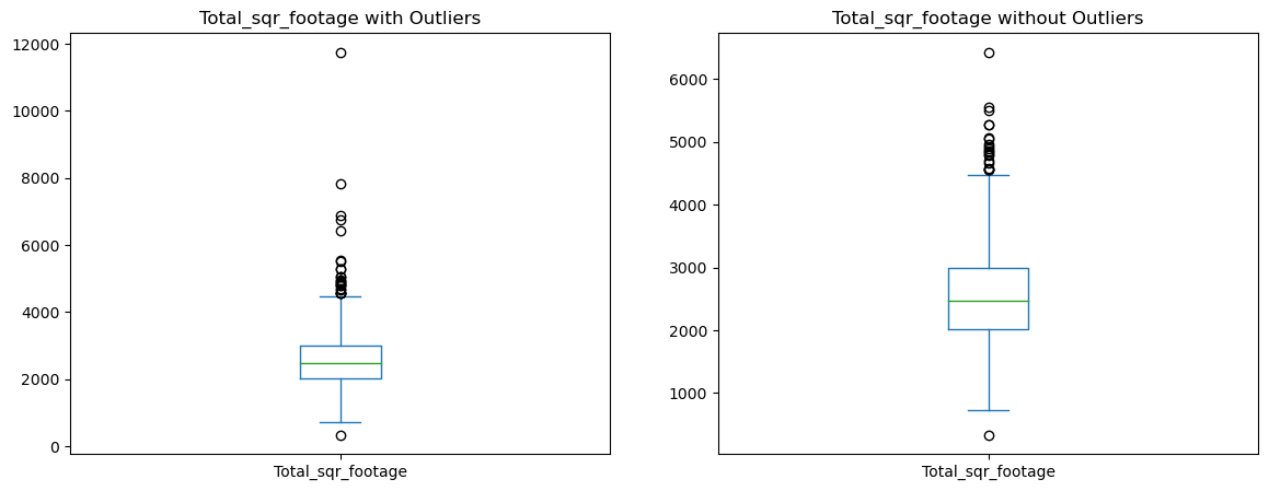
Now we can deal with outliers. Let’s start off with Total_sqr_footage. First, we will see if there are any outliers by drawing a box plot.
Total_sqr_footage has outliers. We will remove the outliers.
plt.figure(figsize=(14, 5))
plt.subplot(1, 2, 1)
df_housing['Total_sqr_footage'].plot.box()
plt.title('Total_sqr_footage with Outliers')
plt.subplot(1, 2, 2)
thr = df_housing['Total_sqr_footage'].mean() + 5*df_housing['Total_sqr_footage'].std()
df_noTSFout = df_housing[df_housing['Total_sqr_footage'] < thr]
df_noTSFout['Total_sqr_footage'].plot.box()
plt.title('Total_sqr_footage without Outliers')
Text(0.5, 1.0, 'Total_sqr_footage without Outliers')

plt.figure(figsize=(14, 5))
plt.subplot(1, 2, 1)
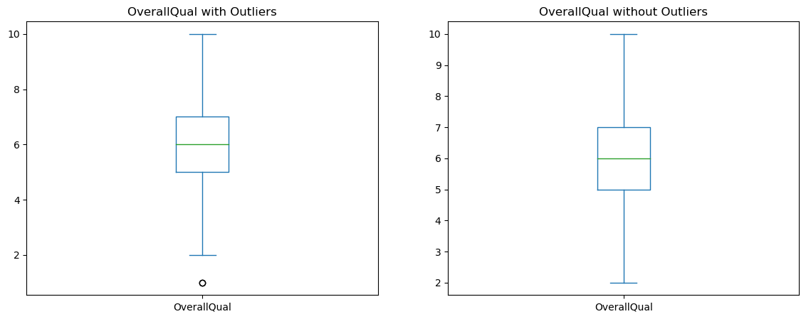
df_noTSFout['OverallQual'].plot.box()
plt.title('OverallQual with Outliers')
plt.subplot(1, 2, 2)
thrOQ = df_noTSFout['OverallQual'].mean() - 3*df_noTSFout['OverallQual'].std()
df_noOQout = df_noTSFout[df_noTSFout['OverallQual'] > thrOQ]
df_noOQout['OverallQual'].plot.box()
plt.title('OverallQual without Outliers')
Text(0.5, 1.0, 'OverallQual without Outliers')
plt.figure(figsize=(14, 5))
plt.subplot(1, 2, 1)
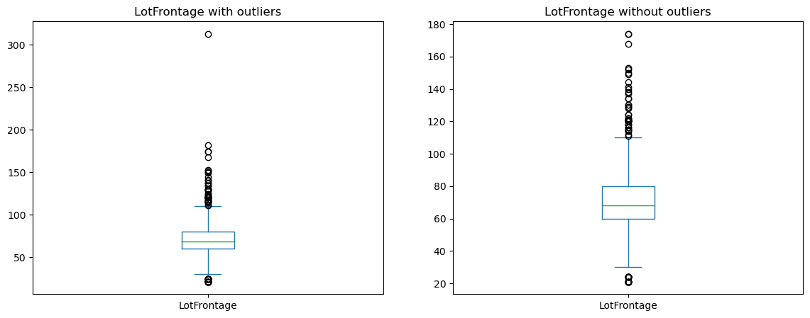
df_noOQout['LotFrontage'].plot.box()
plt.title('LotFrontage with outliers')
plt.subplot(1, 2, 2)
thrLF = df_noOQout['LotFrontage'].mean() + 5*df_noOQout['LotFrontage'].std()
df_noLFout = df_noOQout[df_noOQout['LotFrontage'] < thrLF]
df_noLFout['LotFrontage'].plot.box()
plt.title('LotFrontage without outliers')
Text(0.5, 1.0, 'LotFrontage without outliers')
plt.figure(figsize=(14, 5))
plt.subplot(1, 2, 1)
df_noLFout['SalePrice'].plot.box()
plt.title('SalePrice with outliers')
plt.subplot(1, 2, 2)
thrSP = df_noLFout['SalePrice'].mean() + 5*df_noLFout['SalePrice'].std()
df_final = df_noLFout[df_noLFout['SalePrice'] < thrSP]
df_final['SalePrice'].plot.box()
plt.title('SalePrice without outliers')
Text(0.5, 1.0, 'SalePrice without outliers')
Correlations
Before we start predicting home prices, it’s important that we understand how American homes have changed over the years and how these changes drive prices. With this in mind, we use both statistical methods (correlational coefficients) and visualizations to answer the following questions.
Part a: Although American families are shrinking [2], it is believed that homes have gotten bigger over the years. Support or refute this statement using the dataset.
Part b: Let’s talk home prices. What are home owners willing to pay more for - more living area (in square feet) or a better quality home?
#Solution to part a
yearbyfootage = df_final.groupby('YearBuilt')['Total_sqr_footage'].mean()
yearbyfootage.plot.line()
plt.title('Mean Total_sqr_footage by Year')
Text(0.5, 1.0, 'Mean Total_sqr_footage by Year')

The statement is not correct. As can be seen in the line graph, the average size of the houses has been going up and down over the years. There is no clear trend.
df_final['OverallQual'].describe()
count    1449.000000
mean        6.087647
std         1.351250
min         2.000000
25%         5.000000
50%         6.000000
75%         7.000000
max        10.000000
Name: OverallQual, dtype: float64
df_final['GrLivArea'].describe()
count    1449.000000
mean     1504.359558
std       491.718296
min       438.000000
25%      1128.000000
50%      1458.000000
75%      1774.000000
max      3608.000000
Name: GrLivArea, dtype: float64
To make a comparison, we need to create two dataframes - one for high quality homes and another for homes with large living area. To consider a home high quality, it needs to have an overall quality of higher than what the 75th percentile of homes have. In this case, a home needs to have a quality ranking of higher than 7 to be considered high quality. As for the homes with large living area, we will use the 75th percentile value as the cutoff. Therefore, a home would be considered to have large living area if it had more than 1774 square feet living area.
#Solution to part b
df_highQuality = df_final[df_final['OverallQual'] > 7]
df_largeGrLivArea = df_final[df_final['GrLivArea'] > 1774]
plt.figure(figsize=(14, 5))
plt.subplot(1, 2, 1)
df_highQuality['SalePrice'].plot.box()
plt.subplot(1, 2, 2)
df_largeGrLivArea['SalePrice'].plot.box()
print(df_highQuality['SalePrice'].mean(), df_largeGrLivArea['SalePrice'].mean())
298148.1126126126 251598.68698060943

#Solution to part b: as it can be seen in the two box plots above, on average, people are willing to pay 298148 dollars for high quality homes, whereas they, on average, pay 251598 dollars for homes with large living area. Therefore, it can be concluded that people are willing to pay more for better quality.
Feature Engineering: modifying/transforming existing data
Feature engineering is the process of creating new columns in a dataset by modifying or transforming existing data. These new columns are more amenable to linear regression. Based on this, let’s answer the following question.
There are three categorical columns in our dataset - Neighborhood, BldgType, Street. We will ignore Neighborhood for the time being as there are too many categories (consider this for the bonus question) and we will also ignore Street (you can see why once you do a value counts).
Let us consider the building type column.
Part a: Do you think including the building type will allow us to predict home prices more accurately? Why/Why not?
Part b: There are multiple categories here, so we cannot simply convert this into a 0/1 column. Instead we will attempt something simpler. What do you think is the single building type that is most helpful in making a prediction? Let’s call this T. Create a column called IsT that equals one if the building type is T and is zero otherwise.
#Solution to part a: Yes, including the building type would allow to increase the accuracy of predicting home prices. By including the Building type, we can examine how and to what extend the building type affects the home prices.
Solution to part a: Yes. The building type can be a heplful feature to add to predict home prices more accurately. That’s because building types are usually correlated with the sale price, meaning it is a relevant data to add.
#Solution to part b
df_final['BldgType'].value_counts()
1Fam      1209
TwnhsE     114
Duplex      52
Twnhs       43
2fmCon      31
Name: BldgType, dtype: int64
df_final['Is1Fam'] = 0
df_final.loc[df_final['BldgType']=='1Fam', 'Is1Fam'] = 1
df_final['Is1Fam'].value_counts()
1    1209
0     240
Name: Is1Fam, dtype: int64
Q3: Brute Force Linear Regression
It is natural to think that our linear regression must take into account every single feature in our dataset, right? After all, more data never hurt anybody.
Run a linear regression using all possible features in the dataset (you can exclude feature “Id” and all the categorical features). Report the RMSE and R^2 error.
#When you use train_test_split, do not forget to include random_state = 0
Important: The random_state=0 ensures that even though the training-test split is done randomly, when you run the code multiple times, the final answer does not change. In other words, you don’t want the grader to get a different R^2 error than you.
x_cols = ['LotFrontage', 'Total_sqr_footage','Is1Fam','OverallQual',
          'OverallCond', 'YearBuilt', 'BsmtFullBath', 'FullBath',
         'HalfBath', 'GarageCars', 'PoolArea', 'GrLivArea']
y_col = ['SalePrice']

# Choose features involved in the prediction
dfX = df_final[x_cols]

# Choose column to predict
dfY = df_final[y_col]

# Break the data
X_train, X_test, Y_train, Y_test = train_test_split(dfX, dfY, test_size=0.3,random_state=0)
print('Traning and test data split: ', len(X_train)/len(dfX),':', len(X_test)/len(dfX))

# Create linear regression object
linearRegression = LinearRegression()

# Fit data
linearRegression.fit(X_train, Y_train)

pd.DataFrame(np.transpose(linearRegression.coef_), x_cols, ['Regression Coeffs'])

Y_predicted = linearRegression.predict(X_test)

# Check error metrics
# Mean squared error
meanSquaredError = metrics.mean_squared_error(Y_test, Y_predicted)
print("Mean Squared Error: ", meanSquaredError)

# Mean root squared error
meanRootError = np.sqrt(meanSquaredError)
print("MeanRootError: ", meanRootError)

#Calculate R^2 score, aka goodness of fit
print('r2_score: ', r2_score(Y_test, Y_predicted))
Traning and test data split:  0.6997929606625258 : 0.3002070393374741
Mean Squared Error:  815541017.9977646
MeanRootError:  28557.678792187657
r2_score:  0.8497175477958767
Improving the brute-force regression
You must have noticed by now that the brute-force regression has a reasonable R^2 error. How can we improve upon this? Is that even possible since we’ve already used all of the features up our sleeve?
We will use feature selection. Use the Kendall-Tau correlation coefficient to identify 4 features that are strongly correlated with the outcome variable SalePrice but not necessarily correlated with each other (at least not strongly). Think of these as “diverse features”.
Run a linear regression with just these four features. In other words, the dfX dataframe should only contain 4 columns. What is the R-squared in this case?
Answer (very) briefly on why you think selecting just 4 features gives us an R^2 error that is so close to the actual R^2 error in Q2. In other words, economists always claim that more data is useful but here we see that whether we use 4 features or several, the error is almost identical. Why is this?
df_final.corr('kendall')
| Id | Total_sqr_footage | OverallQual | OverallCond | YearBuilt | GrLivArea | GarageCars | LotFrontage | PoolArea | SalePrice | FullBath | HalfBath | BsmtFullBath | Is1Fam | |
|---|---|---|---|---|---|---|---|---|---|---|---|---|---|---|
| Id | 1.000000 | -0.010322 | -0.026038 | 0.002563 | -0.007005 | -0.001851 | 0.005719 | -0.025947 | 0.030589 | -0.015919 | 0.001254 | 0.000634 | 0.000409 | -0.015457 |
| Total_sqr_footage | -0.010322 | 1.000000 | 0.516230 | -0.164125 | 0.278189 | 0.694093 | 0.462561 | 0.341973 | 0.031686 | 0.638799 | 0.498980 | 0.198112 | 0.126777 | 0.081254 |
| OverallQual | -0.026038 | 0.516230 | 1.000000 | -0.156039 | 0.503391 | 0.457193 | 0.537146 | 0.203064 | 0.023834 | 0.667681 | 0.506974 | 0.261731 | 0.082438 | 0.023974 |
| OverallCond | 0.002563 | -0.164125 | -0.156039 | 1.000000 | -0.331857 | -0.121809 | -0.231307 | -0.070241 | 0.006840 | -0.106866 | -0.246665 | -0.063268 | -0.046623 | 0.167692 |
| YearBuilt | -0.007005 | 0.278189 | 0.503391 | -0.331857 | 1.000000 | 0.185937 | 0.489170 | 0.141747 | -0.013244 | 0.470646 | 0.434699 | 0.196919 | 0.130299 | -0.106705 |
| GrLivArea | -0.001851 | 0.694093 | 0.457193 | -0.121809 | 0.185937 | 1.000000 | 0.398457 | 0.283694 | 0.033482 | 0.541137 | 0.534302 | 0.353478 | 0.001683 | 0.075491 |
| GarageCars | 0.005719 | 0.462561 | 0.537146 | -0.231307 | 0.489170 | 0.398457 | 1.000000 | 0.286107 | 0.002290 | 0.567890 | 0.479772 | 0.213123 | 0.131624 | 0.016188 |
| LotFrontage | -0.025947 | 0.341973 | 0.203064 | -0.070241 | 0.141747 | 0.283694 | 0.286107 | 1.000000 | 0.044042 | 0.313255 | 0.202592 | 0.089943 | 0.069210 | 0.295824 |
| PoolArea | 0.030589 | 0.031686 | 0.023834 | 0.006840 | -0.013244 | 0.033482 | 0.002290 | 0.044042 | 1.000000 | 0.041009 | 0.017636 | 0.002987 | 0.045007 | 0.026200 |
| SalePrice | -0.015919 | 0.638799 | 0.667681 | -0.106866 | 0.470646 | 0.541137 | 0.567890 | 0.313255 | 0.041009 | 1.000000 | 0.514277 | 0.277556 | 0.182433 | 0.110582 |
| FullBath | 0.001254 | 0.498980 | 0.506974 | -0.246665 | 0.434699 | 0.534302 | 0.479772 | 0.202592 | 0.017636 | 0.514277 | 1.000000 | 0.147492 | -0.061127 | -0.096115 |
| HalfBath | 0.000634 | 0.198112 | 0.261731 | -0.063268 | 0.196919 | 0.353478 | 0.213123 | 0.089943 | 0.002987 | 0.277556 | 0.147492 | 1.000000 | -0.046796 | 0.045494 |
| BsmtFullBath | 0.000409 | 0.126777 | 0.082438 | -0.046623 | 0.130299 | 0.001683 | 0.131624 | 0.069210 | 0.045007 | 0.182433 | -0.061127 | -0.046796 | 1.000000 | -0.042243 |
| Is1Fam | -0.015457 | 0.081254 | 0.023974 | 0.167692 | -0.106705 | 0.075491 | 0.016188 | 0.295824 | 0.026200 | 0.110582 | -0.096115 | 0.045494 | -0.042243 | 1.000000 |
# Choose features involved in the prediction
dfX = df_final[['Total_sqr_footage', 'OverallQual', 'GarageCars','GrLivArea']]

# Choose column to predict
dfY = df_final['SalePrice']

# Break the data
X_train, X_test, Y_train, Y_test = train_test_split(dfX, dfY, test_size=0.3,random_state=0)
print('Traning and test data split: ', len(X_train)/len(dfX),':', len(X_test)/len(dfX))

# Create linear regression object
linearRegression = LinearRegression()

# Fit data
linearRegression.fit(X_train, Y_train)

pd.DataFrame(linearRegression.coef_, dfX.columns, ['Regression Coeffs'])

Y_predicted = linearRegression.predict(X_test)

# Check error metrics
# Mean squared error
meanSquaredError = metrics.mean_squared_error(Y_test, Y_predicted)
print("Mean Squared Error: ", meanSquaredError)

# Mean root squared error
meanRootError = np.sqrt(meanSquaredError)
print("MeanRootError: ", meanRootError)

#Calculate R^2 score, aka goodness of fit
print('r2_score: ', r2_score(Y_test, Y_predicted))
Traning and test data split:  0.6997929606625258 : 0.3002070393374741
Mean Squared Error:  954286764.3922529
MeanRootError:  30891.532244164468
r2_score:  0.8241504082640767
What is important when it comes to building an accurate predictive model is not the number of features selected, but rather whether those features that are highly correlated with the target feature have been selected. This is because some features can be irrelevant and decrease the model’s predictive accuracy.
Data analysis Interpretation
Based on your analysis, what do you think are the most informative features (columns), i.e., what are potential buyers most influenced by when they buy a house? Name at least two features (and at most 4) for this answer.
Note: You may have run multiple regressions by this point. Use any of them to answer this question.
# Choose features involved in the prediction
dfX = df_final[['Total_sqr_footage', 'OverallQual']]

# Choose column to predict
dfY = df_final['SalePrice']

# Break the data
X_train, X_test, Y_train, Y_test = train_test_split(dfX, dfY, test_size=0.3,random_state=0)
print('Traning and test data split: ', len(X_train)/len(dfX),':', len(X_test)/len(dfX))

# Create linear regression object
linearRegression = LinearRegression()

# Fit data
linearRegression.fit(X_train, Y_train)

pd.DataFrame(linearRegression.coef_, dfX.columns, ['Regression Coeffs'])

Y_predicted = linearRegression.predict(X_test)

# Check error metrics
# Mean squared error
meanSquaredError = metrics.mean_squared_error(Y_test, Y_predicted)
print("Mean Squared Error: ", meanSquaredError)

# Mean root squared error
meanRootError = np.sqrt(meanSquaredError)
print("MeanRootError: ", meanRootError)

#Calculate R^2 score, aka goodness of fit
print('r2_score: ', r2_score(Y_test, Y_predicted))
Traning and test data split:  0.6997929606625258 : 0.3002070393374741
Mean Squared Error:  1000962061.8565565
MeanRootError:  31637.984478417024
r2_score:  0.8155493961684328
Total_sqr_footage and OverallQual are the two most informative features.
Training Test Split
In all our experiments so far, we have used a 70:30 split for the training and test data. We need to verify if this 70:30 split is sacred or if other ratios are also okay. To answer this question, run the linear regression in Q2 again with a a) 50:50 split and b) 90:10 split.
What are the RMSE and R^2 error in both cases. Based on your experiments, can you conclude which of the three (50:50, 70:30, 90:10) is the best ratio for a training-test split.
x_cols = ['LotFrontage', 'Total_sqr_footage','Is1Fam','OverallQual',
          'OverallCond', 'YearBuilt', 'BsmtFullBath', 'FullBath',
         'HalfBath', 'GarageCars', 'PoolArea', 'GrLivArea']
y_col = ['SalePrice']

# Choose features involved in the prediction
dfX = df_final[x_cols]

# Choose column to predict
dfY = df_final[y_col]

# Break the data
X_train, X_test, Y_train, Y_test = train_test_split(dfX, dfY, test_size=0.5,random_state=0)
print('Traning and test data split: ', len(X_train)/len(dfX),':', len(X_test)/len(dfX))

# Create linear regression object
linearRegression = LinearRegression()

# Fit data
linearRegression.fit(X_train, Y_train)

pd.DataFrame(np.transpose(linearRegression.coef_), x_cols, ['Regression Coeffs'])

Y_predicted = linearRegression.predict(X_test)

# Check error metrics
# Mean squared error
meanSquaredError = metrics.mean_squared_error(Y_test, Y_predicted)
print("Mean Squared Error: ", meanSquaredError)

# Mean root squared error
meanRootError = np.sqrt(meanSquaredError)
print("MeanRootError: ", meanRootError)
#Calculate R^2 score, aka goodness of fit
print('r2_score: ', r2_score(Y_test, Y_predicted))
Traning and test data split:  0.4996549344375431 : 0.5003450655624568
Mean Squared Error:  787958597.3313371
MeanRootError:  28070.600231048447
r2_score:  0.8475411139959701
x_cols = ['LotFrontage', 'Total_sqr_footage','Is1Fam','OverallQual',
          'OverallCond', 'YearBuilt', 'BsmtFullBath', 'FullBath',
         'HalfBath', 'GarageCars', 'PoolArea', 'GrLivArea']
y_col = ['SalePrice']

# Choose features involved in the prediction
dfX = df_final[x_cols]

# Choose column to predict
dfY = df_final[y_col]

# Break the data
X_train, X_test, Y_train, Y_test = train_test_split(dfX, dfY, test_size=0.1,random_state=0)
print('Traning and test data split: ', len(X_train)/len(dfX),':', len(X_test)/len(dfX))

# Create linear regression object
linearRegression = LinearRegression()

# Fit data
linearRegression.fit(X_train, Y_train)

pd.DataFrame(np.transpose(linearRegression.coef_), x_cols, ['Regression Coeffs'])

Y_predicted = linearRegression.predict(X_test)

# Check error metrics
# Mean squared error
meanSquaredError = metrics.mean_squared_error(Y_test, Y_predicted)
print("Mean Squared Error: ", meanSquaredError)

# Mean root squared error
meanRootError = np.sqrt(meanSquaredError)
print("MeanRootError: ", meanRootError)
#Calculate R^2 score, aka goodness of fit
print('r2_score: ', r2_score(Y_test, Y_predicted))
Traning and test data split:  0.8999309868875086 : 0.10006901311249138
Mean Squared Error:  802695104.7805327
MeanRootError:  28331.874360524274
r2_score:  0.8527449288758877
Based on this experiment, it looks like the 90:10 split produces the best r2_score.
Improve upon the R-squared
The two teams with the best R-squared errors (highest) will receive one bonus point each if they can improve upon the error in Q2/Q3. If more than two teams can beat the R^2 error, then they will all receive extra 0.5 points.
Hint 1: How can we incorporate Neighborhood as a feature?
Hint 2: Try to identify features that are correlated with SalePrice but not so much with the other features, i.e., our input features need to be complementary to each other.
Hint 3: Start with the best R^2 error from Q2 or Q3 and try adding or removing a single feature.
Please don’t waste too much time on this question. Your final answer must use a 70:30 split.
from sklearn.preprocessing import LabelEncoder
labelencoder = LabelEncoder()
df_final['Neighborhood'] = labelencoder.fit_transform(df_final['Neighborhood'])
df_final['BldgType'] = labelencoder.fit_transform(df_final['BldgType'])
df_final.loc[df_final['Street'] == 'Pave', 'Street'] = 1
df_final.loc[df_final['Street'] == 'Grvl', 'Street'] = 0
df_final.head()
| Id | Neighborhood | Total_sqr_footage | OverallQual | OverallCond | YearBuilt | GrLivArea | GarageCars | LotFrontage | PoolArea | SalePrice | Street | BldgType | FullBath | HalfBath | BsmtFullBath | Is1Fam | |
|---|---|---|---|---|---|---|---|---|---|---|---|---|---|---|---|---|---|
| 0 | 1 | 5 | 2566 | 7 | 5 | 2003 | 1710 | 2 | 65.0 | 0 | 208500 | 1 | 0 | 2 | 1 | 1 | 1 |
| 1 | 2 | 24 | 2524 | 6 | 8 | 1976 | 1262 | 2 | 80.0 | 0 | 181500 | 1 | 0 | 2 | 0 | 0 | 1 |
| 2 | 3 | 5 | 2706 | 7 | 5 | 2001 | 1786 | 2 | 68.0 | 0 | 223500 | 1 | 0 | 2 | 1 | 1 | 1 |
| 3 | 4 | 6 | 2473 | 7 | 5 | 1915 | 1717 | 3 | 60.0 | 0 | 140000 | 1 | 0 | 1 | 0 | 1 | 1 |
| 4 | 5 | 15 | 3343 | 8 | 5 | 2000 | 2198 | 3 | 84.0 | 0 | 250000 | 1 | 0 | 2 | 1 | 1 | 1 |
x_cols = ['LotFrontage', 'Total_sqr_footage','OverallQual', 'OverallCond', 'BsmtFullBath',
          'YearBuilt', 'GarageCars', 'FullBath',
           'GrLivArea', 'Neighborhood', 'Street', 'BldgType']
y_col = ['SalePrice']

# Choose features involved in the prediction
dfX = df_final[x_cols]

# Choose column to predict
dfY = df_final[y_col]

# Break the data
X_train, X_test, Y_train, Y_test = train_test_split(dfX, dfY, test_size=0.3,random_state=0)
print('Traning and test data split: ', len(X_train)/len(dfX),':', len(X_test)/len(dfX))

# Create linear regression object
linearRegression = LinearRegression()

# Fit data
linearRegression.fit(X_train, Y_train)

pd.DataFrame(np.transpose(linearRegression.coef_), x_cols, ['Regression Coeffs'])

Y_predicted = linearRegression.predict(X_test)

# Check error metrics
# Mean squared error
meanSquaredError = metrics.mean_squared_error(Y_test, Y_predicted)
print("Mean Squared Error: ", meanSquaredError)

# Mean root squared error
meanRootError = np.sqrt(meanSquaredError)
print("MeanRootError: ", meanRootError)
#Calculate R^2 score, aka goodness of fit
print('r2_score: ', r2_score(Y_test, Y_predicted))
Traning and test data split:  0.6997929606625258 : 0.3002070393374741
Mean Squared Error:  757280619.9116006
MeanRootError:  27518.732163956982
r2_score:  0.8604533848629967